Bragg Edge Raw Sample and Powder
Notebook name: bragg_edge_raw_sample_and_powder.ipynb
Description
Start the notebook
If you need help accessing this notebook, check the How To > Start the python notebooks tutorial.
How to Use It?
Select your IPTS
Check the full tutorial here
Select Raw Data Input Folder
Select the folder containing the full sample tof data. The program will automatically try to locate the time spectra file in this folder. If not found, you will need to locate it next.

Select Open Beam Input Folder
Just like it was done for the sample data, select the open beam folder. The notebook will let you know if the sample and ob folders have the same number of files.
Select Background Region
In order to improve the normalization, you have the option to select a region of interest (ROI) in the radiographs of the sample. Make sure that if you select a region, this region is away from the sample, and only contain the background.
Select how many random files to use to select ROI
The first widget allows you to select how many images to use (those will be summed into a single view) to define that region of interest. The higher the number of images used, the longer the next user interface will take to show up. Usually the default value is a good compromise and is high enough to get a good idea of the position of the sample.
Select background region in integrated image
Check the ROI selection tool tutorial to learn how to use that tool.
Normalize Data
The program will use the sample and ob loaded, and the optional background ROI, to normalized the data.
Powder element(s) to use to compare the Bragg edges
This is where you can define one, or more element to use to compare the Bragg edges with.
You can choose any element from the following list:
‘C (diamond)’ ‘C (graphite)’ ‘Si’ ‘Ge’ ‘AlAs’ ‘AlP’ ‘AlSb’ ‘GaP’ ‘GaAs’ ‘GaSb’ ‘inconel’ ‘InP’ ‘InAs’ ‘InSb’ ‘MgO’ ‘SiC’ ‘CdS’ ‘CdSe’ ‘CdTe’ ‘ZnO’ ‘ZnS’ ‘PbS’ ‘PbTe’ ‘BN’ ‘BP’ ‘CdS’ ‘ZnS’ ‘AlN’ ‘GaN’ ‘InN’ ‘LiF’ ‘LiCl’ ‘LiBr’ ‘LiI’ ‘NaF’ ‘NaCl’ ‘NaBr’ ‘NaI’ ‘KF’ ‘KCl’ ‘KBr’ ‘KI’ ‘RbF’ ‘RbCl’ ‘RbBr’ ‘RbI’ ‘CsF’ ‘CsCl’ ‘CsI’ ‘Al’ ‘Fe’ ‘Ni’ ‘Cu’ ‘Mo’ ‘Pd’ ‘Ag’ ‘W’ ‘Pt’ ‘Au’ ‘Pb’ ‘TiN’ ‘ZrN’ ‘HfN’ ‘VN’ ‘CrN’ ‘NbN’ ‘TiC’ ‘ZrC0.97’ ‘HfC0.99’ ‘VC0.97’ ‘NC0.99’ ‘TaC0.99’ ‘Cr3C2’ ‘WC’ ‘ScN’ ‘LiNbO3’ ‘KTaO3’ ‘BaTiO3’ ‘SrTiO3’ ‘CaTiO3’ ‘PbTiO3’ ‘EuTiO3’ ‘SrVO3’ ‘CaVO3’ ‘BaMnO3’ ‘CaMnO3’ ‘SrRuO3’ ‘YAlO3’
This is based on a library we developed called BraggEdge.
To enter more than 1 element, use a colon to separate them. Run the next cell to check if the element is part of the list.

Select Sample ROI
This is where you define the position (ROI) of your sample on the radiographs. Only the counts within that region will be used in the rest of the notebook.
Check the ROI selection tool tutorial to learn how to use that tool.
Define Experiment Setup
Those information will be needed to convert the time of flight values into lambda. Make sure you used the right units
- dSD (distance source detector) in meters
- detector offset in micro seconds
Calculate Bragg Edge Data
Just run this cell to let the notebook convert TOF information into lambda and prepare the data to compare them with the un-strained, powder, Bragg edges.
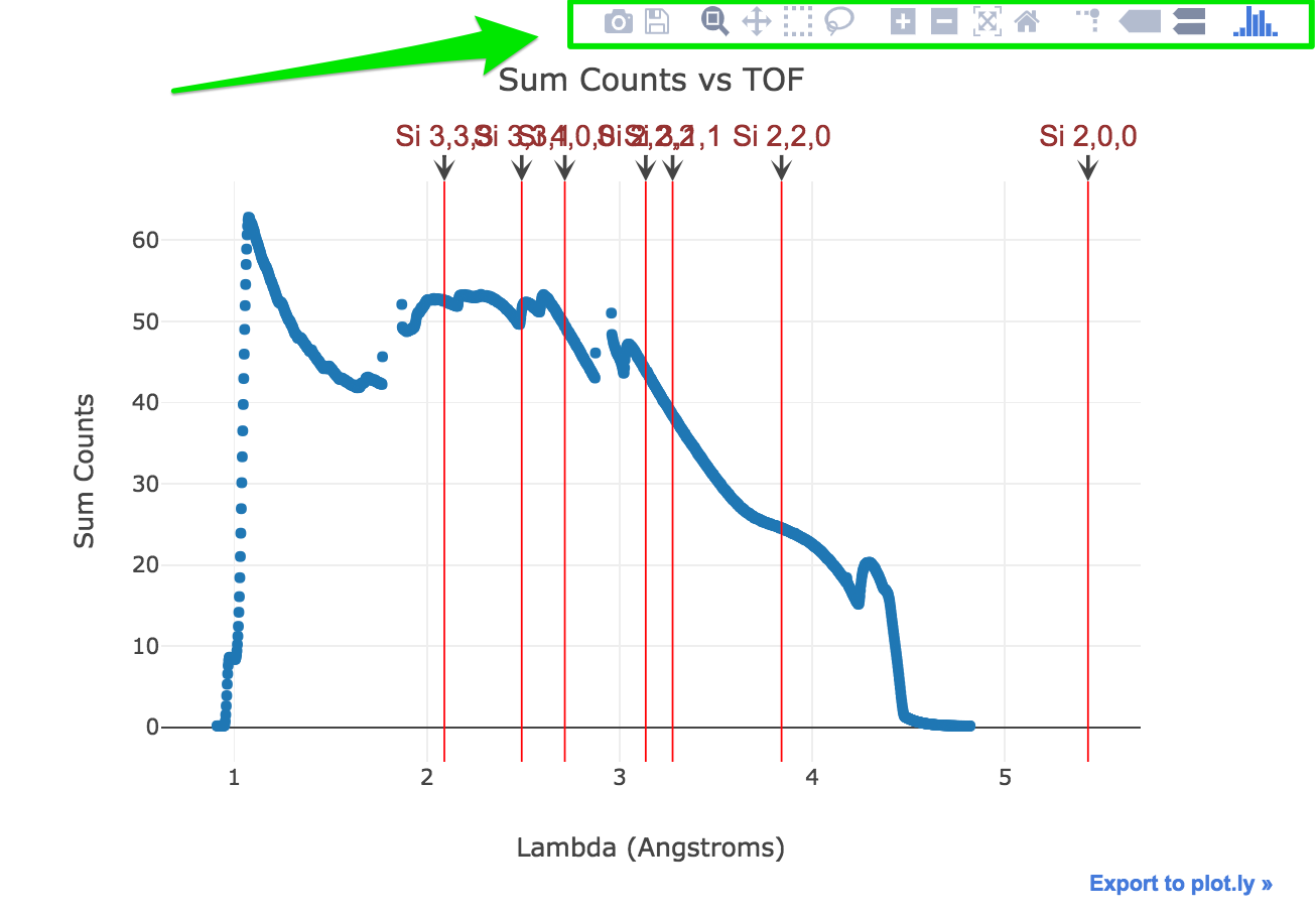
Display Bragg Edges vs Signal
Sample signal and un-strained Bragg edges of elements selected will be displayed on the same plot.

Feel free to play with the iPlot widgets (above the plot) to zoom, pan, … etc
Export Data
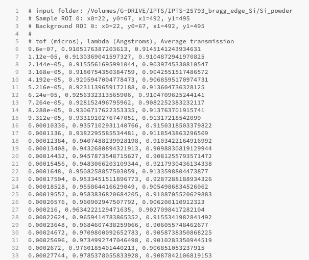
Transmission versus Lambda
You can now export into an ascii file the average transmission vs Lambda (and tof) The ascii file created will have the following format
  #  input sample folder
  #  list of region of interest used to define sample position
  #  list of region of interest used to define background position
  #
  #  tof (micros), lambda (Angstroms), Average transmission
  #  all data in 3 columns format
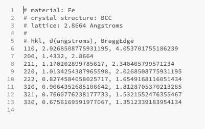
Power Bragg edge table
You can also export the Bragg edges values of the various elements you selected